
On a production line the accuracy of a defect classifier depends more on label quality and on optical-setup stability than on the choice of algorithm. It is a conclusion that no one chasing the best model wants to hear, but it comes back every time a prototype moves from the bench to in-line inspection.
Context and problem
Automated visual quality control is nothing new: rule-based machine-vision systems have been around for decades and work well when the defect has a defined shape — a missing hole, a dimension out of tolerance. Things get harder when the defect is statistical — a scratch, a texture variation, an inclusion — and its appearance shifts with lighting, part position and tool wear. There, a fixed threshold yields either too many false alarms or too many escapes.
With learning the problem changes in kind: instead of writing the acceptance rule by hand, you gather a set of labelled images — conforming or non-conforming, split by defect type when needed — and train a classifier. The gain is real when defect variability is wide, but the cost shifts: no longer engineering the rule, but building and maintaining the dataset.
Architecture
A typical pipeline today, in 2014, has three distinct stages.
Feature extraction. From the raw image you compute descriptors that summarise texture, edges and local statistics. The common ones remain Local Binary Patterns for texture, Haralick descriptors over the grey-level co-occurrence matrix, the Histograms of Oriented Gradients (HOG) of Dalal and Triggs for edge structure, and Lowe’s SIFT descriptors when scale and rotation invariance are needed. The choice of features is already domain knowledge: for a scratch the gradient direction is what counts; for an inclusion, the local intensity statistics.
Classification. A supervised model is trained on the features. Two families cover almost every industrial case of the period: Support Vector Machines with an RBF kernel and Breiman’s Random Forests, robust to noisy features and with a variable-importance measure useful for working out which descriptors really count. Both come in mature tooling: scikit-learn 0.14 (August 2013) for the Python prototype, OpenCV 2.4 for feature extraction and for C++ deployment on the cell.
Decision and threshold. The classifier output is a probability, not a verdict. The acceptance threshold is a process parameter of its own, to be tuned against the asymmetric cost of errors: in many settings an escape — a defect classified as conforming — costs orders of magnitude more than a false alarm, and the threshold should be shifted accordingly.
Deep convolutional neural networks have given notable results on generic image recognition — the system of Krizhevsky, Sutskever and Hinton won ILSVRC 2012, bringing top-5 error from 26% to 15%, and the ILSVRC 2013 winners dropped below 12%. But those results rest on millions of labelled images. On a line that produces a few dozen genuine rejects a day, putting together a dataset of that scale is not practicable, and the feature-plus-classifier pipeline remains the sensible choice.
The critical point
The recurring mistake is to take the accuracy measured in validation for the performance expected in-line. Three factors erode it systematically.
The first is class imbalance: conforming parts are the overwhelming majority, and a classifier that almost always predicts them reaches very high accuracy while detecting nothing. The right metric is not accuracy but the precision/recall pair on the defect class, read off an explicit confusion matrix.
The second is leakage between training and test: if images from the same batch, the same part or the same acquisition session end up in both training and validation, the model learns contingent conditions by heart — a reflection, a shade of background — and the estimate turns optimistic. The split must be made by physical unit and by session, not by individual image.
The third is domain shift: lighting changes, the optics get dirty, the supplier of the raw blank varies, the tool wears. The features computed on those images drift, and a model trained on the setup of three months ago degrades without a single error showing up in the logs. What is needed is monitoring of the feature distribution in operation, not just the one-off metric at acceptance.
Implications
In practice the model is the smallest part of the system. The bulk of the investment sits in the acquisition subsystem — controlled, repeatable lighting, part fixturing, calibration — and in the labelling process, which wants a competent operator and a written, shared acceptance criterion. When two inspectors label the same part differently, no algorithm recovers that inconsistency: it leaves it as irreducible noise in the Bayes limit.
The same holds for predictive models on process parameters. Correlating temperature, pressure and speed with finished-product quality can be done, but a correlation on observational data is not control: a parameter may be associated with rejects because it is a symptom of a common cause, not because acting on it reduces rejects. The distinction between association and intervention lever should be kept explicit before a model goes into production. Across the two tracks — defect detection by visual analysis and predictive models on process parameters — noze gathers its experience in a dedicated insight: https://www.noze.it/en/insights/ml-industry/.
Limits
A trained classifier recognises only the defects present in the dataset. A new failure mode — an unseen contamination, a defect that arrives with a change of supplier — is not flagged as anomalous: it lands in the nearest class, often “conforming”. Novelty-detection or one-class methods file the problem down in part, but with false-alarm rates that are hard to tolerate on a line.
Then there is explainability. A Random Forest gives feature importance; an SVM with a kernel does not. Where a wrong reject opens disputes or rework costs, being able to justify a classification — which image region, which descriptor — is a genuine requirement, to be weighed when choosing the model, not afterwards.
- https://www.cs.toronto.edu/~kriz/imagenet_classification_with_deep_convolutional.pdf
- https://www.stat.berkeley.edu/~breiman/randomforest2001.pdf
- https://lear.inrialpes.fr/people/triggs/pubs/Dalal-cvpr05.pdf
- https://www.cs.ubc.ca/~lowe/papers/ijcv04.pdf
- https://scikit-learn.org/stable/whats_new/v0.14.html
- https://docs.opencv.org/2.4/
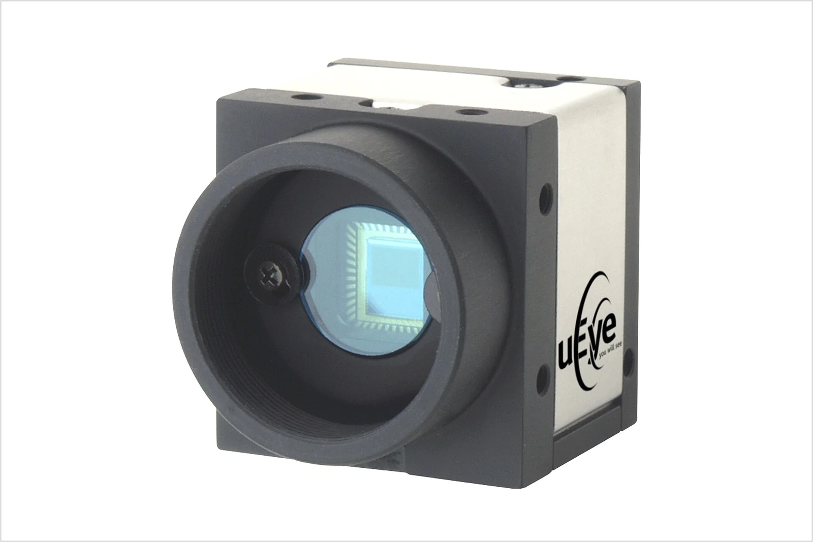
Cover image: IDS uEye industrial machine vision camera with USB connection, close-up of the body and lens mount — photo by Lg123456, CC BY-SA 4.0 — https://commons.wikimedia.org/wiki/File:Ids-machine-vision-cameras-usb2-2004.jpg